Best practice to VLookup values in Excel

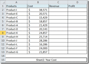
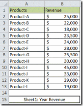
Vlookup is a function that helps you search for a value in a range of cells and return the same or a different value from that range on the same row. To make the picture clearer, let’s take a scenario in which Zaid, an accountant working in XYZ Company, has an Excel file of two sheets; Year Revenue, and Year Cost of a list of XYZ products. Zaid is trying to combine the two sheets’ revenue and cost figures to calculate the profit for each product.

It’s obvious that Zaid has two options so that he can calculate each product’s Profit (Revenue minus Cost):

1. search for each product’s revenue in sheet1 and place it in its corresponding cell in sheet2, or

2. search for each product’s cost in sheet2 and place it in its corresponding cell in sheet1

Zaid elected to follow option 1 and added two extra columns in sheet2; Revenue and Profit.

      Figure (1)                                         Figure (2)

It’s worth mentioning that my experience with people who usually get incorrect results when applying the Vlookup function is that they either:

a. forget to ‘fix’ the lookup range (table array, as referred to in the Vlookup formula) using the dollar sign ($), and/or

b. try to lookup values of different data types. E.g. they lookup Invoice number between two sheets in which it is of Number format in one and of text format in the other.

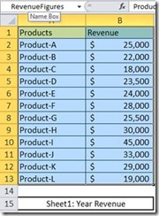
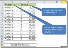
To avoid the first problem, which is the most common, try to name the range of cells in which you need to search for Revenue values. To do this, select the range of cells that covers all data (including headers) in sheet1 and type any name in the Name Box (do not use space in the Name Box). I will name the range RevenueFigures (figure 3).

Figure (3)

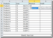
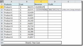
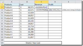
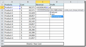
Back to our scenario, we’re ready to apply the Vlookup formula in sheet2 to lookup the first Revenue value. I like and do prefer writing formulas than using the Insert Function, so I will write ‘=vl’ in cell C2 and Excel will narrow down my search to ‘VLOOKUP’ function as shown in figure (4). Hitting the TAB keyboard button will insert the function showing the arguments you need to insert to lookup the Revenue value of Product-I from sheet1 (figure 5).

Figure (4)                                                      Figure (5)

First, you need to specify the value in sheet2 that will be looked up from sheet1 which is captioned as lookup_value in the vlookup function. Select this value by moving the cursor to cell A2. This means that you need to search for Product-I in sheet1.

Figure (6)

Obviously, you have to specify the range of cells in which you need Excel to search for the lookup value, which is the second argument captioned table_array. Type a comma to end the first argument then type the first letters of the sheet1 Range name you previously defined until Excel finds it for you. Great Excel! (Figure 7).

Figure (7)

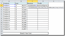
Well, now you’ve got to identify the value in the Range that you need Excel to return to sheet2 if the lookup value has been found in sheet1. I.e. you need to tell Excel to return the Revenue figure of Product-I from sheet1 and place it in cell C2 in sheet2. This is achieved by specifying the col_index_num. This is the column number of the return value reference to the lookup value in the Range. So, we need to return the value in column number 2 (Revenue).

Figure (8)                                                        Figure (9)

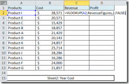
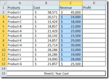
The last argument to complete the Vlookup formula is either TRUE or FALSE. Use FALSE to get the exact match (recommended always) and TRUE to get approximate match. Close the function with “)” and hit the return keyboard key to get the result. Then apply the formula to the rest of products by copy/paste.

Figure (10)                                                          Figure (11)

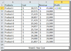
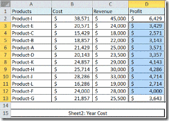
By this Zaid will be able to calculate each product’s profit by deducting the cost from the looked up revenue.

Figure (12)                                                          Figure (13)

After applying the Vlookup function to your data I recommend to always have a couple checks to the figures by taking samples of looked up values and comparing them to those in the searched Range.

Customize Excel Ribbon and make your macros default commands

I believe that efficient use of Microsoft Office Excel has a tremendous effect on office work efficiency. With this blog I start a series of powerful tips and tricks that I’m sure will change the way you perform some tasks and will make using Excel a sort of fun!

If you have created a macro to do a specific job regularly, have you ever wondered how you can make the macro available in any Excel file you open (even new ones)? Moreover, have you ever wished to have all of your own, customized macros appear in a new, separate tab in the Excel Ribbon? Then follow the below steps that walk you through an example to list a macro (Profitability macro in this example) in a new tab (My Macros tab) in the Excel 2010 Ribbon.

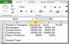
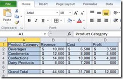
When the macro, so called Profitability, runs it performs some calculations (Profit and Grand Total) and reformats the range of data in terms of cell background color and number formatting as shown below.

(1) Before running Profitability macro (2) after running Profitability macro

The default Ribbon tabs found in Excel 2010 are the ones show in figure (3). In this example we are going to add a new customized tab named “My Macros”. The My Macros tab will include the Profitability macro that we need to be available by default in any Excel file we open afterwards.

(3) Ribbon in Excel 2010 before adding customized tabs

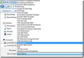
First, you have to make sure you save the original macro as Excel Add-in (figure 4) then you close and reopen Excel.

Figure (4) saving the macro as Excel Add-in file

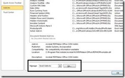
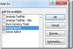
Then you need to enable the add-in by going to the Backstage view (File menu)>Options>Add-Ins (figure 5). Select Excel Add-ins from the Manage dropdown list and hit Go. From the Add-Ins window select the new add-in you created for the macro and hit OK (figure 6).

Figure (5)                                                    Figure (6)

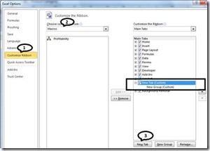
By this your macro is accessible by any Excel file you open but we need to make it appear as any other command in the Ribbon tabs. Go to the Backstage view and hit the Options button, then hit the Customize Ribbon button on left pane.

Select Macros option from the ‘Choose Commands From’ dropdown list. All macros available in the workbook will be listed as shown in figure (7).

The next step is to create a new tab to be displayed in the Ribbon. Hit the New Tab button in the bottom right side of the window. A new tab will be automatically added under the Main Tabs list as shown in the figure.

Figure (7)

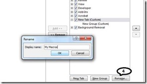
Rename the new tab to any name you like, ‘My Macros’ for instance, by hitting the Rename button. Write the new name in the Display Name text box that appears (Figure 8). The new tab will be changed to ‘My Macros’ as soon as you hit the OK button.

Figure (8)

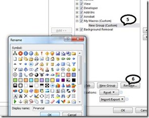
Any new tab would have to have at least one Group of commands. You can elect to change the name of the Group to another name that best describes the group of commands you wish to insert in the Group. Let’s select ‘Financial’ as a Group name (Figure 9).

Figure (9)

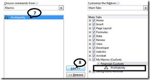
Now, it’s time to add your macro (Profitability) to the Financial Group under the new My Macros tab. Make sure the Financial Group is selected in the right pane, then select the macro you want to add from the left pane and hit the Add button in the middle of the window (figure 10).

Figure (10)

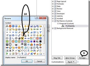
By this you will have a new tab with the hierarchy of My Macros>Financial>Profitability. You may want to change the symbol of the macro to another meaningful one, e.g. select the dollar sign ($) as a symbol for the Profitability macro (figure 11)

Figure (11)

By hitting the OK but to close the Excel Options window you will see your new tab shown in the Ribbon with the hierarchy you built as shown in figure 12.

Figure (12)

By this you have made your own automatic procedure (macro) available for any file you open with Excel and that is placed as a command item in your own Ribbon tab.